Kang IFN-β PBMC: MOFA-FLEX from R to MOFA2
Maximilian Nuber
2026-03-09
kang-analysis.RmdOverview
This vignette demonstrates an end-to-end MOFA-FLEX workflow entirely in R:
-
Load the Kang et al. (2018) PBMC IFN-β stimulation
dataset from
muscData. - Preprocess with standard Bioconductor tools (scran / scuttle).
-
Bridge the resulting
SingleCellExperiment— a subclass ofSummarizedExperiment— into a PythonAnnDataviasce_to_reticulate_anndata(), using matrix-type-aware dispatch that converts the assay matrix to a NumPy array or a SciPy sparse matrix and applies zero-copy where possible. -
Train a MOFA-FLEX model with
fit_mofaflex(), saving the model to an HDF5 file compatible with MOFA2. - Load the saved model in the MOFA2 R package for downstream analysis.
Required packages
# Bioconductor
library(muscData) # BiocManager::install("muscData")
library(scuttle) # BiocManager::install("scuttle")
library(scran) # BiocManager::install("scran")
library(SingleCellExperiment)

# MofaflexR (this package)
library(MofaflexR)

# Downstream — MOFA2
library(MOFA2) # BiocManager::install("MOFA2")
Load data
muscData::Kang18_8vs8() provides 29,065 PBMCs from eight
donors, each split into a control and an IFN-β–stimulated condition (8 ×
2 = 16 samples).
sce_full <- Kang18_8vs8()
#> see ?muscData and browseVignettes('muscData') for documentation
#> loading from cache
sce_full
#> class: SingleCellExperiment
#> dim: 35635 29065
#> metadata(0):
#> assays(1): counts
#> rownames(35635): MIR1302-10 FAM138A ... MT-ND6 MT-CYB
#> rowData names(2): ENSEMBL SYMBOL
#> colnames(29065): AAACATACAATGCC-1 AAACATACATTTCC-1 ... TTTGCATGGTTTGG-1
#>   TTTGCATGTCTTAC-1
#> colData names(5): ind stim cluster cell multiplets
#> reducedDimNames(1): TSNE
#> mainExpName: NULL
#> altExpNames(0):
# class: SingleCellExperiment
# dim: 35,635 genes × 29,065 cells
# colData names: ind, stim, cluster, cell, multipletsPreprocess
Quality-control filtering
Remove multiplets and low-quality cells before normalisation.
## Remove multiplets and cells without an assigned cell type
sce <- sce_full[, sce_full$multiplets == "singlet" & !is.na(sce_full$cell)]

## Keep cells with ≥ 200 detected genes
qc <- scuttle::perCellQCMetrics(sce)
sce <- sce[, qc$detected >= 200]

cat(sprintf("After QC: %d genes × %d cells\n", nrow(sce), ncol(sce)))
#> After QC: 35635 genes × 24562 cells
Normalisation
Log-normalise using pooling-based size factors from scran.
set.seed(42)
# clusters <- scran::quickCluster(sce)
# sce      <- scran::computeSumFactors(sce, clusters = clusters)
sce <- scuttle::logNormCounts(sce)

assayNames(sce) # should include "logcounts"
#> [1] "counts"    "logcounts"
Select highly variable genes
Retain the 3,000 most variable genes to keep the model tractable.
dec <- scran::modelGeneVar(sce)
hvgs <- scran::getTopHVGs(dec, n = 3000)
sce_hvg <- sce[hvgs, ]

cat(sprintf("Using %d HVGs from %d cells.\n", nrow(sce_hvg), ncol(sce_hvg)))
#> Using 3000 HVGs from 24562 cells.
Convert to AnnData
sce_to_reticulate_anndata() bridges the selected assay
from the SingleCellExperiment (a
SummarizedExperiment subclass) to a Python
anndata.AnnData object using matrix-type-aware
conversion:
-
Sparse matrices (e.g.
dgCMatrix) are converted to a matching SciPy sparse format (csc_matrixfor CSC,csr_matrixfor CSR, etc.) and zero-copy is used for the backing slot arrays where possible. -
Dense matrices (e.g.
dgeMatrix, basematrix) are converted to NumPy arrays, with zero-copy attempted via the R-to-NumPy buffer protocol. - All
colDatacolumns are forwarded toadata.obs;rowDatagoes toadata.var. - The assay (originally features × cells) is transposed once to
AnnData’s expected
obs × vars = cells × featureslayout.
The logcounts assay produced by
scuttle::logNormCounts() is typically stored as a sparse
matrix, so the returned adata$X will be a SciPy sparse
matrix (CSR after transposition).
adata <- sce_to_reticulate_anndata(
    sce_hvg,
    assay = "logcounts"
)
adata
#> ReticulateAnnData object with n_obs × n_vars = 24562 × 3000
#>     obs: 'ind', 'stim', 'cluster', 'cell', 'multiplets', 'sizeFactor'
#>     var: 'ENSEMBL', 'SYMBOL'
The stim column in adata$obs
("ctrl" / "stim") will be used by MOFA-FLEX to
split cells into two groups.
Train a MOFA-FLEX model
Key choices:
-
group_by = "stim"— split cells into ctrl and stim groups using thestimcolumn inobs. -
subset_var = NULL— HVGs were already selected; skip thehighly_variablefilter. -
save_path— write the trained model to an HDF5 file. -
mofa_compat = "full"— save in MOFA2-readable format. - View name will be
rna(automatic when wrapping a single AnnData).
## Output path — adjust to a stable directory in your project
output_dir <- file.path("results", "mofaflex")
dir.create(output_dir, recursive = TRUE, showWarnings = FALSE)
model_path <- file.path(output_dir, "kang_mofaflex.hdf5")
model <- fit_mofaflex(
    data = adata,
    data_options = list(
        # group_by           = "stim",
        scale_per_group    = TRUE,
        subset_var         = NULL,
        plot_data_overview = FALSE
    ),
    model_options = list(
        n_factors    = 5L,
        weight_prior = "Horseshoe"
    ),
    training_options = list(
        max_epochs             = 5000L,
        early_stopper_patience = 50L,
        seed                   = 42L,
        device                 = "cuda",  # or "cpu" if no GPU is available
        save_path              = model_path
    ),
    mofa_compat = "full"  # write a MOFA2-readable HDF5 file
)
Compute time. On a modern CPU this typically converges in a few minutes thanks to early stopping.
Load the model in MOFA2
Because the model was saved with mofa_compat = "full",
the HDF5 file contains all MOFA2-compatible weight and factor matrices.
Use the load_mofaflex_model() wrapper (which handles minor
HDF5-format differences between mofaflex and MOFA2
automatically) to load it.
mofa <- load_mofaflex_model(model_path)
#> Warning in .quality_control(object, verbose = verbose): The model contains highly correlated factors (see `plot_factor_cor(MOFAobject)`).
#> We recommend that you train the model with less factors and that you let it train for a longer time.

## Attach sample metadata so colour_by aesthetics work.
## MOFA2 requires a 'sample' column matching the model's cell IDs.
cells_per_group <- MOFA2::samples_names(mofa)
meta <- do.call(rbind, lapply(names(cells_per_group), function(grp) {
    cells <- cells_per_group[[grp]]
    sdf <- as.data.frame(SummarizedExperiment::colData(sce_hvg)[cells, , drop = FALSE])
    data.frame(
        sample = cells, group = grp, sdf,
        check.names = FALSE, stringsAsFactors = FALSE
    )
}))
MOFA2::samples_metadata(mofa) <- meta
mofa
#> Trained MOFA with the following characteristics:
#>  Number of views: 1
#>  Views names: rna
#>  Number of features (per view): 3000
#>  Number of groups: 1
#>  Groups names: group_1
#>  Number of samples (per group): 24562
#>  Number of factors: 5
Variance explained
MOFA2::plot_variance_explained(mofa, max_r2 = 0.1)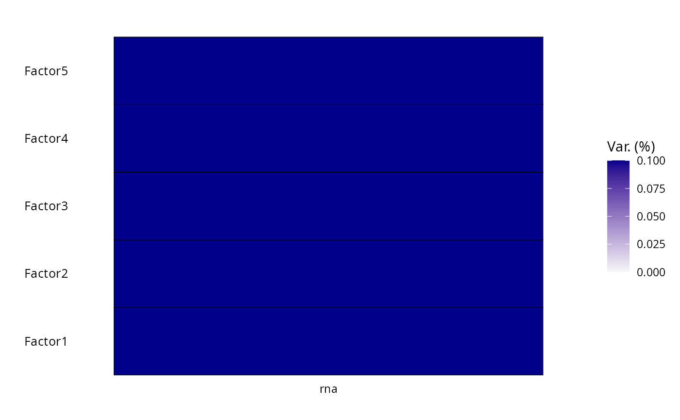
Variance explained per factor and group.
Factor scores
MOFA2::plot_factor(
    mofa,
    factors = 1:5,
    color_by = "stim",
    add_violin = FALSE,
    dodge = TRUE,
    add_boxplot = TRUE
)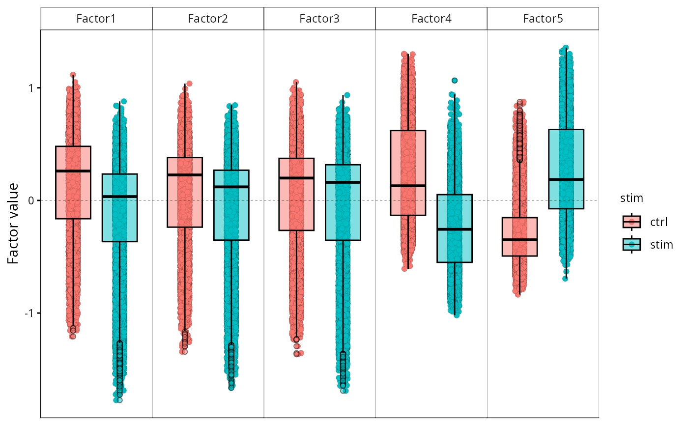
Factor scores coloured by stimulation condition.
Top feature weights
MOFA2::plot_top_weights(
    mofa,
    view      = "rna",
    factor    = 5,
    nfeatures = 10
)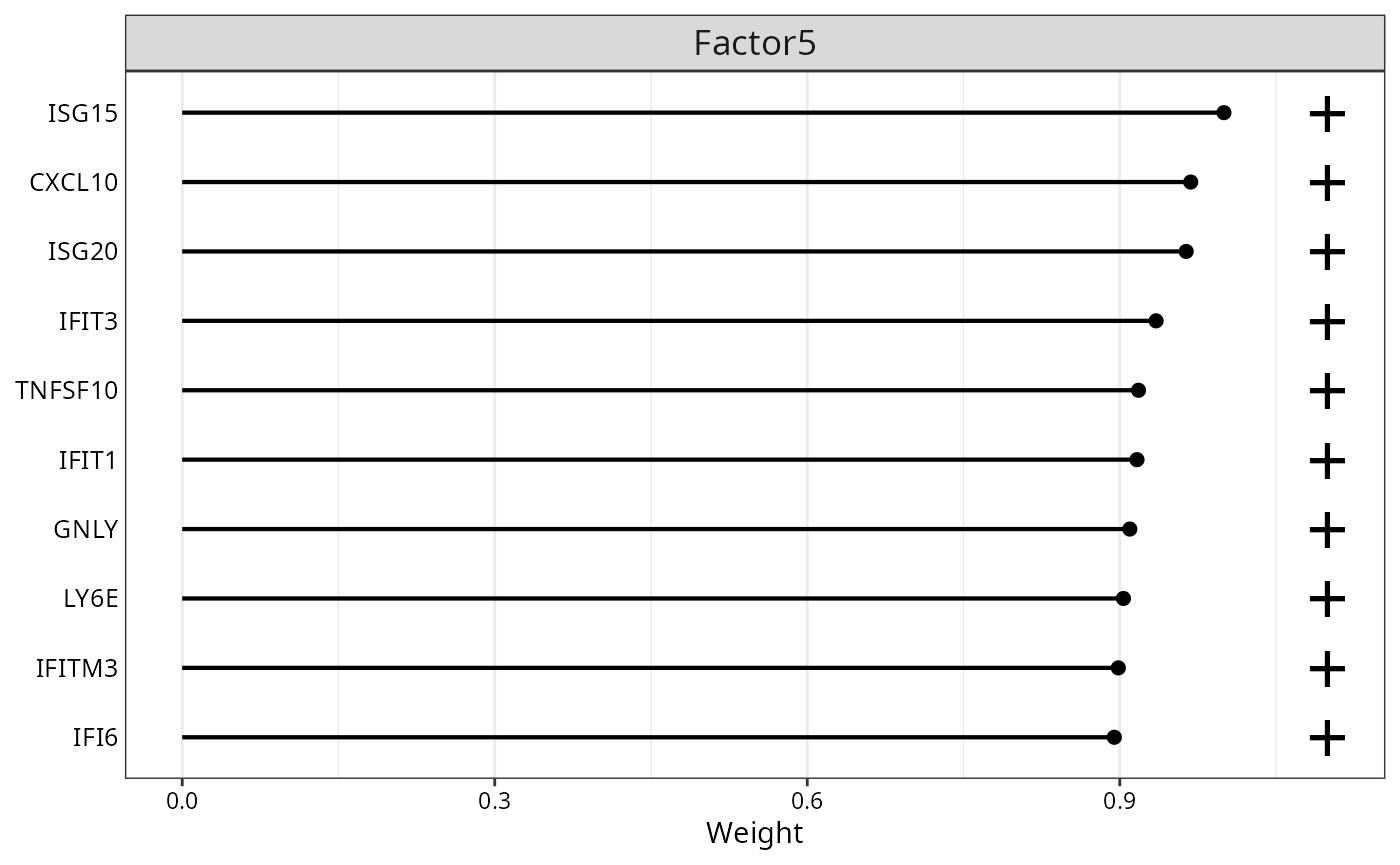
Top 10 feature weights for Factor 1.
factors <- MOFA2::get_factors(mofa, factors = 1:5)
df <- cbind(
    factors$group_1,
    as.data.frame(SummarizedExperiment::colData(sce_hvg)[rownames(factors$group_1), ])
)
umaps <- uwot::umap(factors$group_1, n_neighbors = 15, min_dist = 0.1, metric = "cosine")
df <- cbind(df, UMAP1 = umaps[, 1], UMAP2 = umaps[, 2])
ggplot2::ggplot(df, ggplot2::aes(x = UMAP1, y = UMAP2, color = stim)) +
    ggplot2::geom_point(size = 0.5, alpha = 0.6) +
    ggplot2::theme_minimal() +
    ggplot2::labs(title = "UMAP of MOFA-FLEX factors coloured by stimulation condition")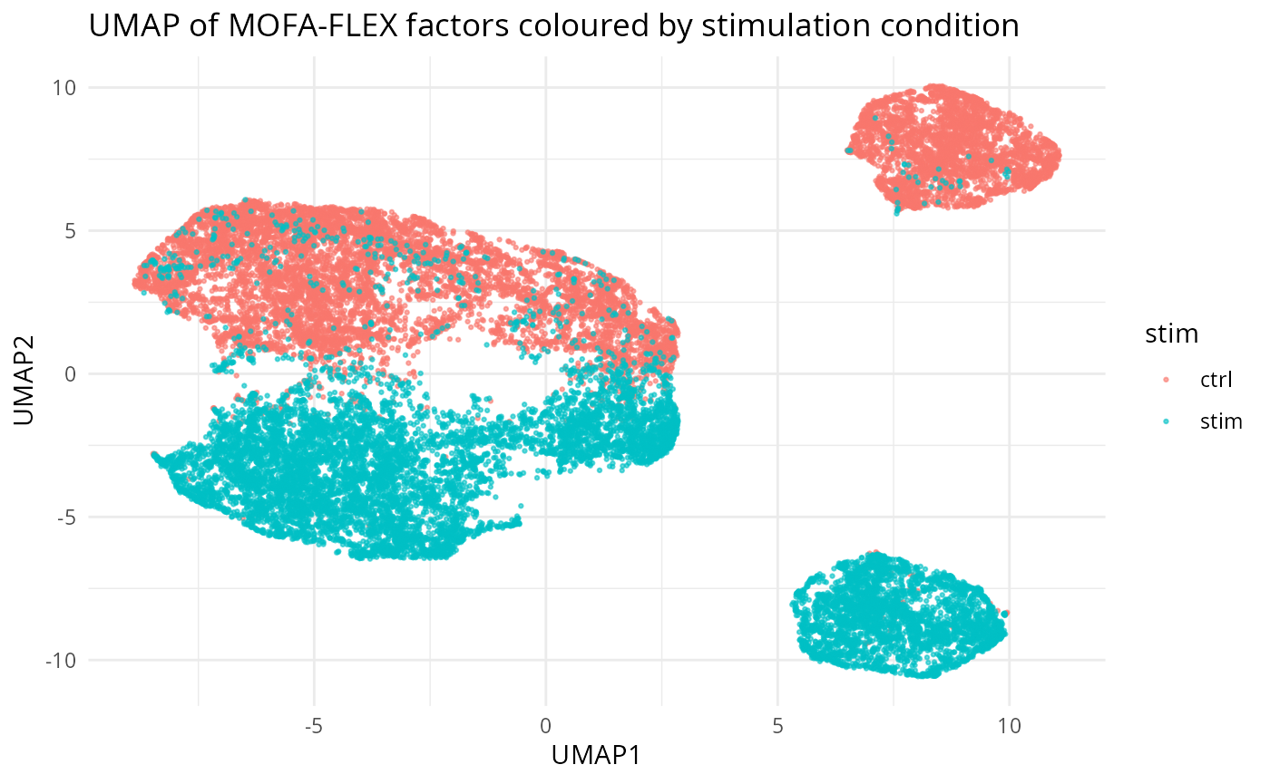
UMAP of MOFA-FLEX factor scores coloured by stimulation condition.
Alternatively, use basilisk to run MOFAFlex in a separate Python
process. The model is saved to disk anyway and loaded with MOFA2. If
setBasiliskShared(TRUE), the Python model is loaded into
the current R session.
basilisk::setBasiliskFork(TRUE) # use forked processes for parallelism (Linux/Mac only)
basilisk::setBasiliskShared(FALSE) # share the same Python environment across processes (saves memory)

output_dir <- file.path("results", "mofaflex")
dir.create(output_dir, recursive = TRUE, showWarnings = FALSE)
model_path <- file.path(output_dir, "kang_mofaflex.hdf5")

with_mofaflex_env({
  # sce_to_reticulate_anndata uses matrix-type-aware dispatch:
  # the logcounts assay (typically sparse) is converted to SciPy sparse;
  # zero-copy is used for the backing data arrays where possible.
  adata <- MofaflexR::sce_to_reticulate_anndata(sce_hvg, assay = "logcounts")
  MofaflexR::fit_mofaflex(
    data = adata,
    data_options = list(scale_per_group = TRUE, subset_var = NULL, plot_data_overview = FALSE),
    model_options = list(n_factors = 5L, weight_prior = "Horseshoe"),
    training_options = list(max_epochs = 5000L, early_stopper_patience = 50L, seed = 42L,
                            device = "cuda", save_path = model_path),
    mofa_compat = "modelonly"
  )
  return(NULL)
}, sce_hvg = sce_hvg, model_path = model_path)
Session info
sessionInfo()
#> R version 4.5.2 (2025-10-31)
#> Platform: x86_64-pc-linux-gnu
#> Running under: Ubuntu 24.04.4 LTS
#>
#> Matrix products: default
#> BLAS:   /usr/lib/x86_64-linux-gnu/openblas-pthread/libblas.so.3
#> LAPACK: /usr/lib/x86_64-linux-gnu/openblas-pthread/libopenblasp-r0.3.26.so;  LAPACK version 3.12.0
#>
#> locale:
#>  [1] LC_CTYPE=en_US.UTF-8       LC_NUMERIC=C
#>  [3] LC_TIME=de_DE.UTF-8        LC_COLLATE=en_US.UTF-8
#>  [5] LC_MONETARY=de_DE.UTF-8    LC_MESSAGES=en_US.UTF-8
#>  [7] LC_PAPER=de_DE.UTF-8       LC_NAME=C
#>  [9] LC_ADDRESS=C               LC_TELEPHONE=C
#> [11] LC_MEASUREMENT=de_DE.UTF-8 LC_IDENTIFICATION=C
#>
#> time zone: Europe/Berlin
#> tzcode source: system (glibc)
#>
#> attached base packages:
#> [1] stats4    stats     graphics  grDevices utils     datasets  methods
#> [8] base
#>
#> other attached packages:
#>  [1] MOFA2_1.20.2                MofaflexR_0.0.1
#>  [3] scran_1.38.1                scuttle_1.20.0
#>  [5] muscData_1.24.0             SingleCellExperiment_1.32.0
#>  [7] SummarizedExperiment_1.40.0 Biobase_2.70.0
#>  [9] GenomicRanges_1.62.1        Seqinfo_1.0.0
#> [11] IRanges_2.44.0              S4Vectors_0.48.0
#> [13] MatrixGenerics_1.22.0       matrixStats_1.5.0
#> [15] ExperimentHub_3.0.0         AnnotationHub_4.0.0
#> [17] BiocFileCache_3.0.0         dbplyr_2.5.2
#> [19] BiocGenerics_0.56.0         generics_0.1.4
#> [21] BiocStyle_2.38.0
#>
#> loaded via a namespace (and not attached):
#>   [1] RColorBrewer_1.1-3   jsonlite_2.0.0       magrittr_2.0.4
#>   [4] farver_2.1.2         corrplot_0.95        rmarkdown_2.30
#>   [7] fs_1.6.6             ragg_1.5.0           vctrs_0.7.1
#>  [10] memoise_2.0.1        htmltools_0.5.9      S4Arrays_1.10.1
#>  [13] forcats_1.0.1        curl_7.0.0           BiocNeighbors_2.4.0
#>  [16] Rhdf5lib_1.32.0      SparseArray_1.10.8   rhdf5_2.54.1
#>  [19] sass_0.4.10          bslib_0.10.0         htmlwidgets_1.6.4
#>  [22] basilisk_1.22.0      desc_1.4.3           plyr_1.8.9
#>  [25] httr2_1.2.2          cachem_1.1.0         igraph_2.2.2
#>  [28] lifecycle_1.0.5      pkgconfig_2.0.3      anndataR_1.0.2
#>  [31] rsvd_1.0.5           Matrix_1.7-4         R6_2.6.1
#>  [34] fastmap_1.2.0        digest_0.6.39        AnnotationDbi_1.72.0
#>  [37] RSpectra_0.16-2      dqrng_0.4.1          irlba_2.3.7
#>  [40] textshaping_1.0.4    RSQLite_2.4.6        beachmat_2.26.0
#>  [43] labeling_0.4.3       filelock_1.0.3       httr_1.4.8
#>  [46] abind_1.4-8          compiler_4.5.2       withr_3.0.2
#>  [49] bit64_4.6.0-1        S7_0.2.1             BiocParallel_1.44.0
#>  [52] DBI_1.3.0            HDF5Array_1.38.0     rappdirs_0.3.4
#>  [55] DelayedArray_0.36.0  bluster_1.20.0       tools_4.5.2
#>  [58] otel_0.2.0           glue_1.8.0           h5mread_1.2.1
#>  [61] rhdf5filters_1.22.0  grid_4.5.2           Rtsne_0.17
#>  [64] cluster_2.1.8.1      reshape2_1.4.5       gtable_0.3.6
#>  [67] tidyr_1.3.2          BiocSingular_1.26.1  ScaledMatrix_1.18.0
#>  [70] metapod_1.18.0       XVector_0.50.0       RcppAnnoy_0.0.23
#>  [73] ggrepel_0.9.7        BiocVersion_3.22.0   pillar_1.11.1
#>  [76] stringr_1.6.0        limma_3.66.0         dplyr_1.2.0
#>  [79] lattice_0.22-7       bit_4.6.0            tidyselect_1.2.1
#>  [82] locfit_1.5-9.12      Biostrings_2.78.0    knitr_1.51
#>  [85] bookdown_0.46        edgeR_4.8.2          xfun_0.56
#>  [88] statmod_1.5.1        pheatmap_1.0.13      stringi_1.8.7
#>  [91] yaml_2.3.12          evaluate_1.0.5       codetools_0.2-20
#>  [94] tibble_3.3.1         BiocManager_1.30.27  cli_3.6.5
#>  [97] uwot_0.2.4           reticulate_1.45.0    systemfonts_1.3.1
#> [100] jquerylib_0.1.4      Rcpp_1.1.1           dir.expiry_1.18.0
#> [103] png_0.1-8            parallel_4.5.2       pkgdown_2.2.0
#> [106] ggplot2_4.0.2        blob_1.3.0           scales_1.4.0
#> [109] purrr_1.2.1          crayon_1.5.3         rlang_1.1.7
#> [112] cowplot_1.2.0        KEGGREST_1.50.0